Sort Data

Data can be sorted from the Data toolbar using Sort menu.

To sort data

1. Select the data that you wish to sort or arrange.

2. Click Data > Sort.

3. The options available under Sort include
   Sort Ascending
   Sort Descending
   Custom Sort

4. Choose to sort data according to your required criterion.

Custom Sort can be used to set your conditions for sorting.

Charts

Charts are tools that help you to visualize and present data in a pictograph form.

Create a Chart

To create a chart

1. Click Insert > Chart.

2. Click the type of the chart required.

3. Select the data range required for the chart.

4. Enter the title of the chart and the X and Y axes titles.

Publish a Chart

1. Click Publish present in the menu when you select the chart

2. Use the code snippet you get to embed or publish your chart.

3. You can also choose to revert the publishing of the chart by clicking Revert Publish found in the menu.

Edit a Chart

1.  Click Edit found in the menu when you select a chart.

2.  You can do your preferred modifications to the chart now. 

Save a Chart as an Image

1. Click More > Save Image present in the menu.

2. The chart is saved as a Portable Network Graphics (.png) image.

Delete a Chart

1. Click More > Delete from the menu.

2. The chart will be deleted.

Formulas

Formulas are used to perform calculations that are required to facilitate the understanding of data. A formula begins with an equal to (=) sign and is followed by syntax that lets you do the required calculations. Formulas can use basic mathematical operations including arithmetic and logical operations.

Insert Function

A function is an inbuilt mathematical operation that helps you perform complicated tasks with relative ease. A function follows the same format as that of a formula and begins with an "equal to" symbol. The syntax varies depending upon the function used.

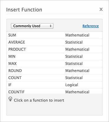
To insert a function

      1.   Click Formulas > Insert Function.

      2.   Choose a function to be inserted from a variety of functions available.

      3.   Enter the addresses of the required cells to be used in the function that fits the syntax of the chosen                 function.

Array Formulas

Array formulas are used when a set or group of numbers are to be considered as input or output data for operators. These formulas are generally applied when the data is used in a group together.

To apply array formulas:

1. Select the cells in which you want the resultant array the result of the output formula to be present.

2. Type the array formula you wish to apply over the array. Like other formulas, an array formula is preceded by an "equals" (=) sign. 

3. You may find it comfortable to name the array you plan to use as input by using Define Name feature found in the context menu.
4. After you enter the formula, press Ctrl + Shift + Enter instead of Enter alone.
5. The array formula will be executed.
                       
   

Cell Reference

There are two ways in which a reference to a cell can be made.

Relative Reference

A formula references a cell relatively if the reference changes when the formula or the function is copied or filled down.

Absolute Reference

A formula references a cell absolutely if the reference to the cell remains constant when the formula or the function is copied or filled down.

To toggle between absolute and relative references:

Absolute reference to a cell is indicated by the use of the symbol "$". To change the reference in a formula

1. Type the required formula or the function in the resultant cell with all the input ranges to achieve your required result.

2. Go to the range that you want to change the reference to and press F4.

3. You can toggle the reference of that range. You can choose only columns, only rows or both rows and columns to be absolute for a cell range.

Recalculate

You can use Recalculate after the data present in the cells have changed. If you click Recalculate, all changes in data are accounted for and formula cells are updated. 

Auto Sum

Use Auto Sum to calculate the sum of the numbers present along a row or a column.

Define Name

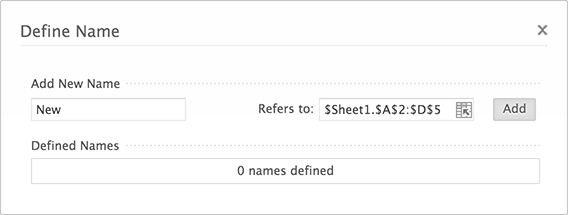
You can define a name for a specific formula that you have created to help you arrive at a result using the given formulas provided in Sheet. To name a formula,

1. Select Formulas > Define Name.

2. Enter a new name for your formula in Add Name data field.

3. Choose what you wish to name. You can choose to name the following
   1. A cell
   2. A range of cells
   3. A specific value
   4. A formula

4. Click Add.

5. You can also view the other user generated formulas that have been named in the same window.
          

Goal Seek

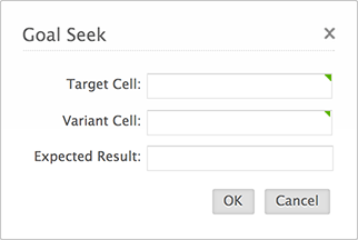
Goal Seek is used to solve for faulty values when the target cell does not provide the expected result. In order to use Goal Seek, follow the given steps.

1. Click Data > Goal Seek.

2. Enter required target cell and the cell that gives you a varying result and not the result you were expecting.

3. The target  cell should be formula cell while the variant cell should not be a formula cell for Goal Seek to work.

4. Click OK to arrive at the required value at the variant cell. 
                                

Solver

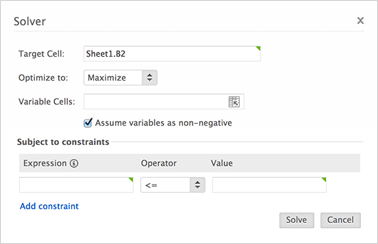
Solver is generally used in order to arrive at an optimum solution for a given value that follows a given set of conditions. Solver currently supports SUM() and SUM PRODUCT() functions. To use Solver, follow the given steps:

1. Choose Data > Solver.

2. A pop-up menu is displayed.
          

3. Choose the target cell, i.e., the cell which contains the value that is to be optimized. It must contain a formula.

4. Choose whether you want the target to be maximized, minimized or to be equal to a specific value.

5. Choose the range of the variable cells, that is, the value of the inputs corresponding to the target cell that is to be optimized. The data present in these cells will be modified according to the optimized value.

6. You can choose the required constraints for optimizing the required cell. The constraint cells should be formula cells. You can choose the constraints to be lesser than, greater than or equal to a chosen value.

7. The target cell is optimized based upon the constraints you specify and you receive a prompt asking you to accept or reject the optimized values. Click OK if you want to accept the optimized values.

Filters

Filters are powerful data analysis tools which are used when a particular set of values need to be analyzed. They are helpful when data need to be sorted and displayed according to a particular condition or criterion.

Select Filter Range

The range in which the filter is to be applied can be selected using any of these methods:

• Choose the column upon which you want to apply the filter.

• Choose the range of the filter automatically by clicking a particular cell which is present in the required cell range.

• Choose the desired filter range by selecting the required cells.

Apply Filter

In order to apply a particular filter, use any of the following methods:
Method 1

After the required filter range is selected, click Filter icon   on the menu bar in Home menu.

Method 2

Click on Data > Filter.

Method 3

Right click on the required range and choose Filter from the contextual menu.

Once you choose the filter option, the columns or the data ranges that have been chosen are added with a triangle that can be used to set the conditions required for filtering.   

Choose the required filtering criterion. The available options include the following:

• Filter by Cell Value - This filter displays only those cells with the selected value. It displays all the values present in the particular column and lets you filter based upon the value.

• Filter by Cell Color - This filter displays those cells with the same background (cell) color.

• Filter by Text Color - It displays only those cells which have text in the selected color.
                            

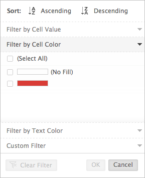
You can choose these options right from the menu bar Filter icon or from the drop down menu  that appears on clicking the triangle. Choose the check box next to the required data cell.

You can also choose to arrange or sort the data according to a particular field.

Custom Filter

There is also an option available to use a filter that satisfies the condition set by you. Click on Custom Filter from the drop down menu from the triangle icon. Custom Filter lets you choose your condition according to which the data must be filtered. 

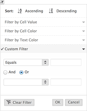
Depending upon the data type chosen, the options that are used to set the conditions or criterion for filtering vary. When the data entry is numerical, the options provided are the following:

• is greater than - displays all numbers greater than the chosen value

• is greater than or equal to - displays numbers greater than or equal to the chosen value

• is less than - displays numbers less than the chosen value

• is less than or equal to - displays numbers less than or equal to the chosen value

If the fields or data to be filtered is made of text fields, you can use the following criterion for filtering.

• equals

• does not equal

• begins with

• does not begin with

• ends with

• does not end with

• contains

• does not contain

• matches

• does not match

If you choose "contains" from the custom menu, it displays all the fields that hold the particular

phrase entered as criterion. You can also use custom filtering with dates as sorting criterion. The options that are available to sort filters in the form of dates include:

• After

• On or after

• Before

• On or before.

The given conditions can be used to sort and display only those dates that follow the set criterion are displayed.

Clear Filter

A filter once applied can be cleared if you want to view the entire spreadsheet again. In order to get the entire sheet back, use the following steps.

1. After a filter is applied, the column to which the filter is applied by a filter icon in the place of a triangle.

2. Click on the filter icon and the context menu, click Clear Filter.

3. Filters that pertain to the chosen column are cleared.

Remove Filter

When filters are enabled in a sheet, the icon  representing filters in the menu bar is displayed. In order to remove filters present in the sheet, click the icon.

Data Validation

Data Validation is useful when the contents of a cell that are to be used as input should pertain to certain conditions or fall within a range. Data validation ensures that data entry remains correct and alerts you if you go wrong in entering data into the spreadsheet.

Create Data Validation

To create a data validation condition for a particular cell, click that cell. If you wish to apply data validation to a range of cells, use drag and drop to select the range of cells.

1. Click Data > Data Validation.

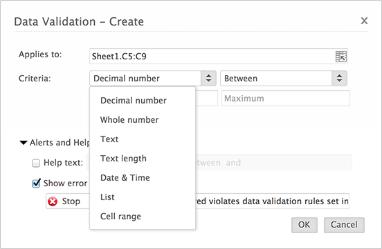
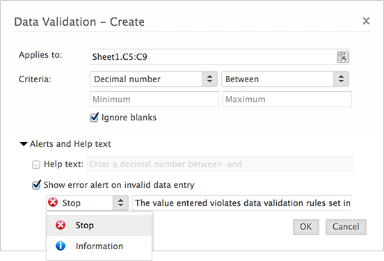
2. You can choose the required range of data validation from the following dialog box.
    

3. The options that are available include the following: Decimal number, Whole number, Text, Text length, Date & Time, List, Cell range. These options are used to set the required condition.

4. You can also use data validation in case of data in the form of text. You can choose a list of values that will be entered into a particular column before using data validation. There will be a drop down list displaying the values you have chosen and you can pick your value from the available list. 
                                 

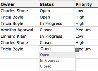
You can also set a legend near a particular cell that uses data validation to regulate its data and a warning error alert when the data validation condition is not followed. It can be done from Create Validation box.

Clear Data Validation

Data validation can be cleared from a cell or a range of cells if found unnecessary. You can clear Data Validation by performing the following steps.

1. Choose the particular cell or the range of cells from which you want to clear data validation.

2. Click Data Validation > Clear Data Validation.

A warning dialog box appears. Click OK and data validation conditions set for that particular cell are removed.

Manage Data Validation

Data Validation conditions that are set all over the spreadsheet can be managed using Manage Data Validation in Data Validation menu.  

Manage Data Validation displays all the cells and cell ranges in which data validation has been put in place. You can choose the settings icon near every validation condition in order to edit it, copy it or clear the available validation.
                                  

Pivot Tables

Pivot Tables are effective data analysis tools. A pivot table helps you organize and summarize the data available to you.

Create Pivot Table

1. Click Data > Pivot > Create Pivot Table.

2. Give the pivot table a title and choose the range of the cells from which the table is to be constructed. You can also choose to describe the table to be created.

3. Click Design Pivot.

Design Pivot

You can design the pivot table according to your specifications.

1.   Drag and drop the required fields in either rows or columns.

2.   Decide which fields appear as rows and which ones appear as columns in the pivot table. Set the data fields as required.

3.   Use Filters to sort and display only the values that meet fixed criterion for better analyzing purposes.

4.   You can view the preview of the pivot table by clicking Click Here to Generate Pivot. Click Done when you want to finalize your pivot table. The generated   table is now displayed in a separate sheet.

5.    If you wish to edit the created pivot table, click Edit Design from the generated pivot table.

Create Pivot Chart

Creating a pivot chart is similar to the creation of a pivot table. A pivot chart is a visual representation of data available in the form of a pivot table.

1. Click Data > Pivot > Create Pivot Chart.

2. Enter the name of the chart and click Design Pivot.

Design Pivot Chart

1. Choose the X-axis, Y- axis, Color and Text required from the available data fields.

2. You can preview the pivot chart to be generated by clicking Click to Generate Preview.

3. Use Edit Design if you want to change fields present in the chart.

View Pivot Reports List

1. Click Data > Pivot > View Pivot Reports List.

2. You can view the list of all pivot charts and pivot tables that have been created present in the workbook.

Delete Pivot Chart

To delete a pivot chart, click Data > Pivot > View Pivot Reports List and click Delete present near the table or the chart you wish to delete.

Link External Data

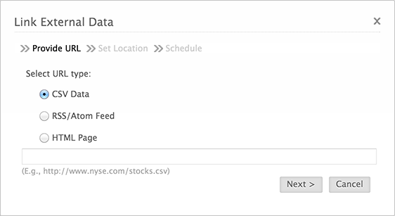
Link External Data can be used to link webpages, CSV Data or RSS Feeds.

To link external data

1. Click Data > Link External Data. The following dialog box appears. 
      

2. Choose the type of data you want to link the spreadsheet to.

3. Set the location where the external data where is to be linked in the spreadsheet. By default, it is set to the cell selected currently.

4. Once you choose the location, set how often the data is to be modified or sourced from the webpage.

5. Click OK.
   

Freeze Panes

Freeze Panes can be used to distinguish the required cells visible while accessing a large amount of data present in the sheet.  

To freeze panes

1. Click View > Freeze Panes.

2. The rows and columns that are present before the currently selected cell are frozen in order to be viewed when the sheet is scrolled down.

Freeze First Row

This feature is used to freeze the first row so that it can be used to compare with other entries present in the spreadsheet. It can be applied from View menu or the context menu.

Freeze First Column

Use Freeze First Column to retain the first column while you scroll along columns to check and verify data.

Unfreeze Panes

Click Unfreeze Panes in View Menu to remove the frozen state of panes.

Text to Columns

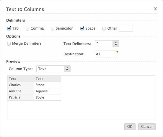
Text to Columns is used to convert text with multiple words into separate columns based on delimiters.

To use Text to Columns

1. Select the required cell or column which consists of the text you want to convert into separate columns.

2. Click Data > Text to Columns. The Text to Columns dialog box appears.
           

3. Choose the delimiters you want to set when text is split into columns.

4. Set the destination of where the new columns are to be placed.

5. Click OK.

Lock Cells

Lock Cells can be used when the owner of a spreadsheet wants to ensure that edited cell ranges or sheets cannot be modified anymore. The owner can also ensure that the ranges or sheets shared with other collaborators can be edited by only by those with access to those cells. 

Lock Cells

Locking Cells and Sheets is available only to owners and co-owners of a particular spreadsheet. If you have been shared the sheet with "Read Only, Read/ Write" or "Read/Comment" permissions, then you cannot use Lock Cells.

To lock a range of cells

1. Select the particular cell or the range of cells that you wish to lock.

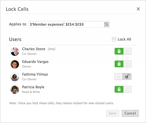
2. Select Data > Lock Cells. The Lock Cells dialog box opens.

3. Choose the collaborators for whom you want to lock the particular cell or the range of cells. The default lock settings for the collaborators will be set at off. You can lock the range of cells by clicking the Lock icon present near the respective collaborator for whom you want wish to restrict access.

4. The Lock icon turns green near the specific collaborator once you have decided to lock those cells for him.

If you lock a specific range of cells, that particular range remains locked by default even for collaborators with whom you share the spreadsheet later once you have locked the range.

Lock Sheet

You can also lock a particular sheet to be made inaccessible to edit for other collaborators.

To lock a sheet

1. Click Data > Lock Sheet.

2. Lock the sheet to those collaborators for whom you wish to lock the cells. The sheet stays locked to newly shared collaborators as well.

3. You can also lock the sheet by right clicking the required sheet and using the context menu.

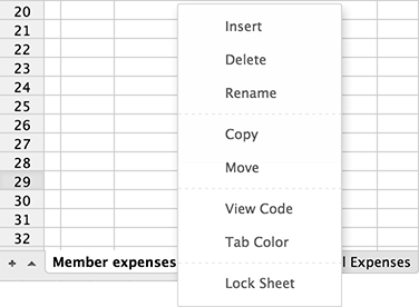
You can unlock both cells and sheets in the same way you had locked them. Select the range of cells that you wish to unlock and click the Lock icon near the collaborators to unlock the ranges or sheets.

Manage Lock Cells

Protection applied to various cells can be managed from Manage Lock Cells dialog box.

To manage lock cells

1. Click Data > Lock > Manage Locked Cells.

2. The dialog box shows all the cell ranges and sheets that have been locked by the user for various collaborators. A green lock icon indicates that the particular cell range has been locked for that specific collaborator.

3. The access to various cell ranges and sheets to various collaborators once provided can be completely managed from this dialog box. You can view, change and delete various lock settings from here.
             

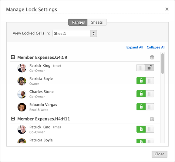
You can lock a specific cell range for a specific collaborator using this dialog box.

Highlight Locked Cells

Highlight Lock Cells lets you highlight and recognize the cells and ranges that have been locked for all collaborators.

To highlight locked cells

1. Click Data > Lock > Highlight Locked Cells.

2. The cells that have been locked for all collaborators will be highlighted and visible now.

3. To bring cells back to their original form, disable Highlight Locked Cells. The cell ranges will be restored back to their original form.
                       

You can view the Manage Lock Settings dialog box by clicking the lock icon present in the range.